ENCAS: Search cascades of neural networks in any model pool
Based on our paper “Evolutionary Neural Cascade Search across Supernetworks” (Best Paper award @ GECCO 2022)
TL;DR Search for cascades of neural networks in model pools of hundreds of models, optionally using Neural Architecture Search to efficiently generate many diverse task-specific neural networks. Get dominating trade-off fronts on ImageNet and CIFAR-10/100, improved ImageNet SOTA (of publicly available models).
Table of contents:
- Motivation
- Background: ensembles & cascades
- Where can we get models for our cascades?
- Background: Neural Architecture Search (NAS)
- Different supernetworks give different trade-off fronts
- How can we search for cascades?
- Experiment setup
- Dominating trade-off front on ImageNet
- NAS-discovered networks are improved by cascading
- Five supernetworks are better than one
- ENCAS outperforms efficient NAS approaches
- Conclusion
Motivation
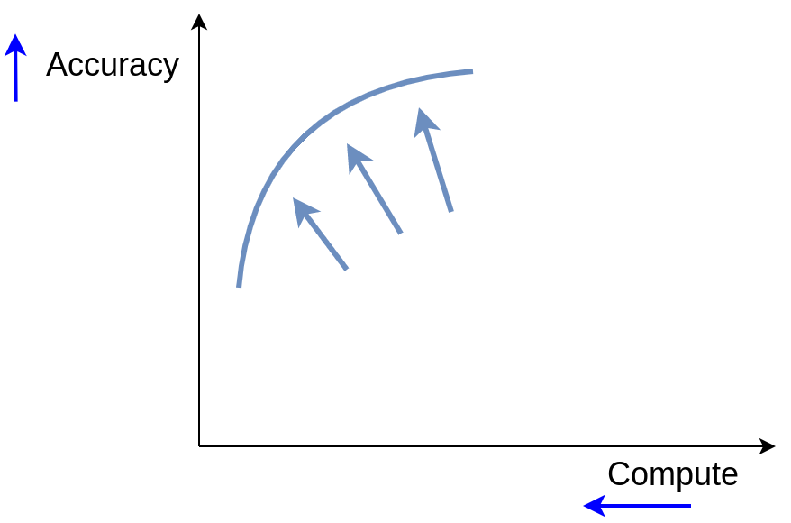
We would always like for our neural networks to be as effective and efficient as possible. In practical terms, it means maximizing some measure of performance (e.g. accuracy) while minimizing some measure of used resources (e.g. FLOPs). So we find ourselves in a multi-objective setting: we want to find a trade-off front of models of varying quality and computation requirements.
Background: ensembles & cascades
One way to improve performance is by combining several models in an ensemble. Let’s say we have two models on our trade-off front:
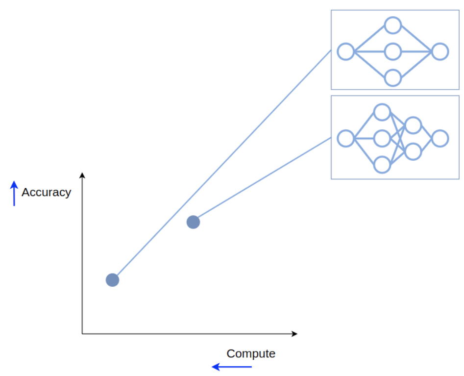
We can create an ensemble by passing the input to both of the models and averaging their outputs. This creates a new point on the trade-off front, with improved performance, but also increased compute requirements.
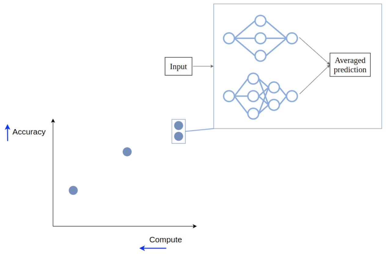
Performance improves because, in terms of the bias-variance tradeoff, ensembling reduce variance: mistakes of different models cancel out. So ensembles benefit from diverse member models: for the mistakes of the ensemble members to cancel out, these mistakes have to be different!
At the same time, efficiency suffers because we are now using two models instead of one, which obviously requires more compute.
But do we actually need to use all the models on all the inputs? Not really, since there exist very simple inputs that can be classified correctly by just one model.
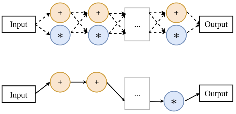
That is the intuition behind cascading. A cascade is just an ensemble with an optional early exit. Let’s return to our two models on the trade-off front and arrange them slightly differently:
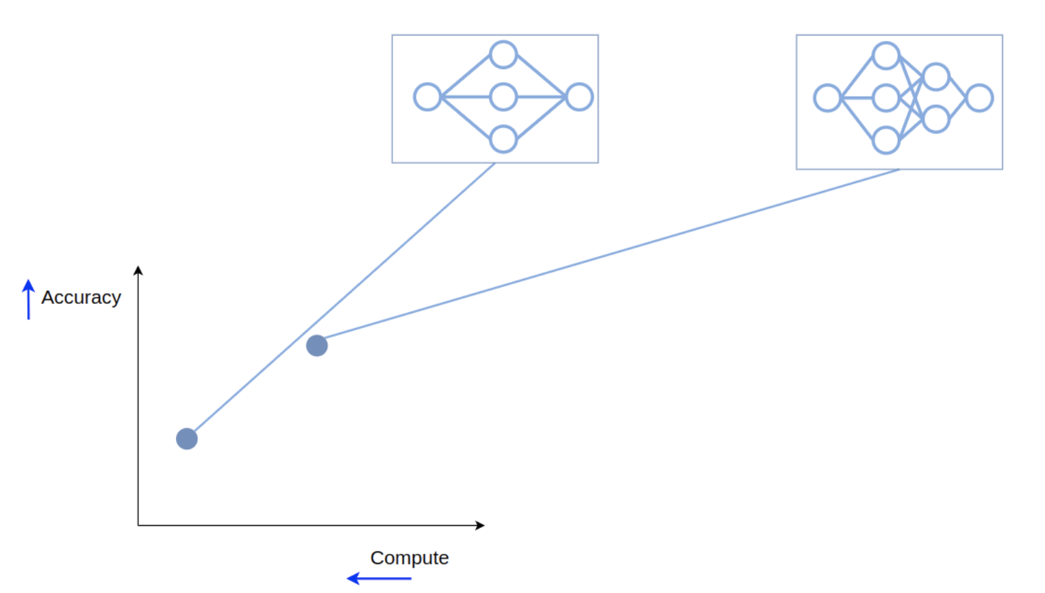
While in an ensemble we passed the input to both of the models, in a cascade we’ll start by passing it only to the first one.
Then we can estimate the confidence of the model’s output - and if it is high enough, stop the computation and return this output as the cascade’s prediction. So if the input is easy, only the first model will be used, and compute won’t be wasted on running the second one.
If, on the other hand, the input is hard, and the first model is not confident, we will pass the input to the second model, and average the outputs of the models, the same way as we did in an ensemble.
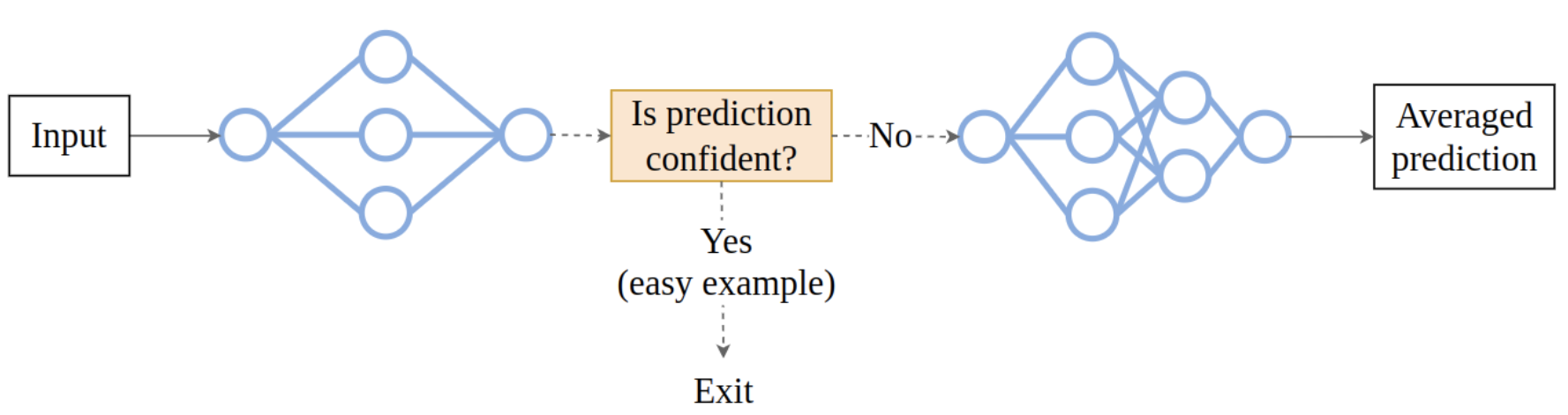
And now we have our cascade, which is again a new point on the trade-off front.
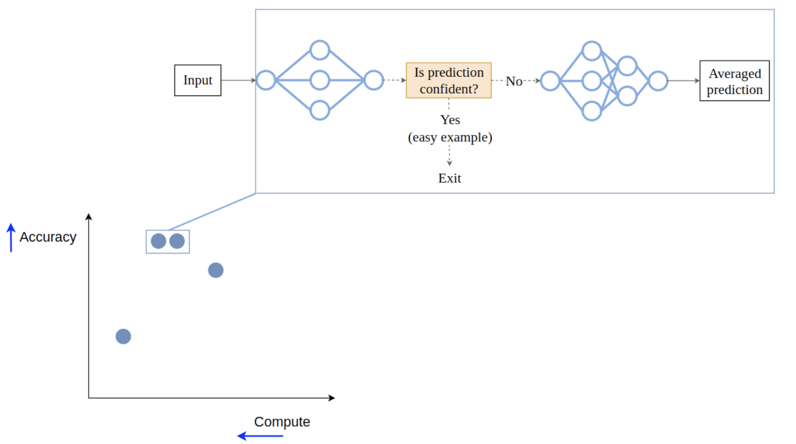
In this case not only has the performance improved (since for hard inputs a cascade is equivalent to an ensemble), but the required compute didn’t grow too much: only the first model is used for all the inputs, and the second one is used rarely, when it’s actually needed. This means that on average we save a lot of compute, and that’s great!
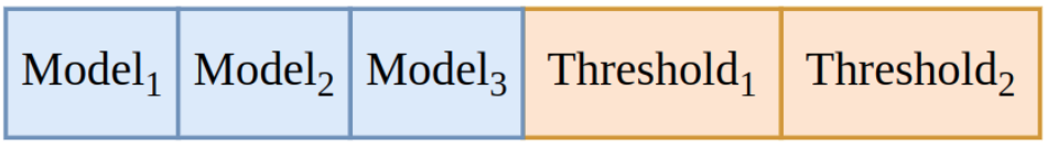
How can we represent a cascade of two models? Well, we need to reference the two used models, and we need to define a confidence threshold for deciding whether to do an early exit:
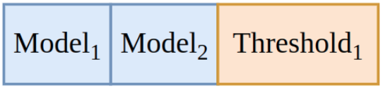
This trivially extends to larger cascades: for a cascade of three models we need two thresholds: the first one to decide whether to stop after the first model; and the second one to decide whether to stop after the second model.
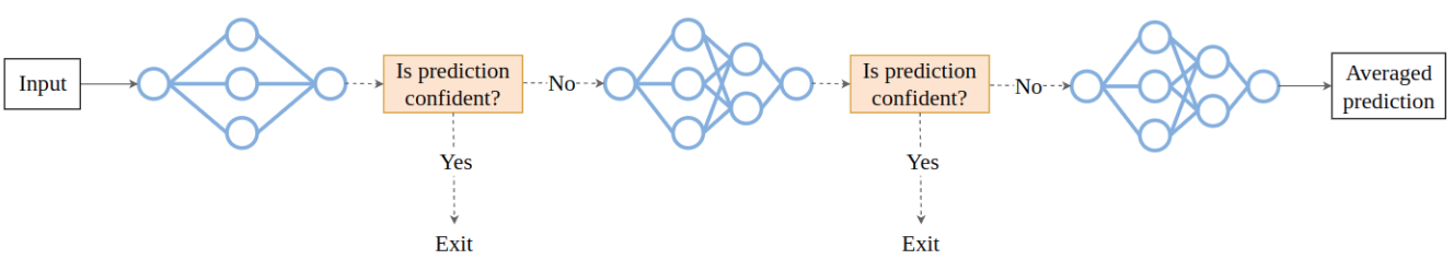
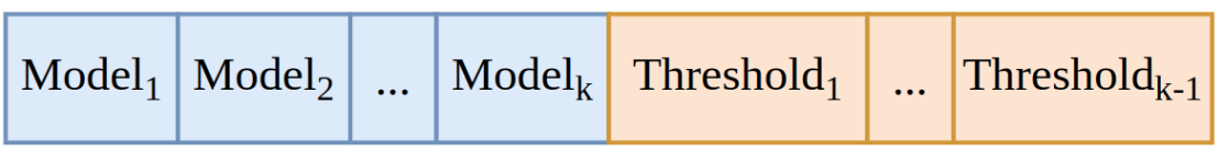
In general, for k models we need k - 1 thresholds.
To sum up, in order to create a cascade we need to select models that work well together, and choose thresholds for deciding on an early exit.
Where can we get models for our cascades?
- Downloading pre-trained models is good if they exist for the dataset you’re interested in, which is often not the case.
- Training many networks manually is possible but labour-intensive, and it’s usually not feasible to train a really large amount of models.
- Neural Architecture Search allows creating hundreds of diverse task-specific models in a single run.
Background: Neural Architecture Search (NAS)
NAS is a paradigm of the automatic search for a task-specific neural network architecture. Architecture can be searched via many approaches, in our work we rely on Evolutionary Algorithms (EAs).
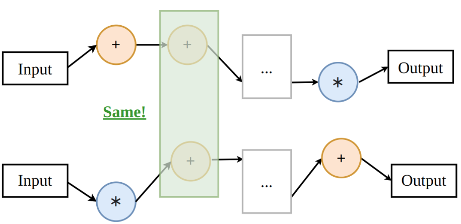
An important direction of NAS research is weight sharing: for the sake of efficiency, not all possible architectures are considered but only those that are subsets of a supernetwork.
In the toy supernetwork below, there are just two possible operations in each position, a subnetwork can use one of them.
This approach is efficient because different subnetworks that use the same operation in the same position can share the weights of this operation (and so they don’t have to be trained from scratch).
In the early supernetwork-based approaches (such as DARTS), the best subnetwork was retrained from scratch after the search. However, there now exist algorithms for training a supernetwork (e.g. OFA, AlphaNet) such that the subnetworks require no retraining - and so if you have a trained supernetwork, you can create hundreds of different models without additional costs!
But the diversity of the models in a supernetwork is restricted by the design of the supernetwork, since all of the subnetworks need to be trained together.
We became curious about how much the results of NAS are influenced by the manual step of choosing a supernetwork, so we investigated what happens with a prominent NAS algorithm called Neural Architecture Transfer (NAT). NAT is a multi-objective NAS algorithm that can adapt a pretrained supernetwork to any task with the help of an EA called NSGA-III.
Different supernetworks give different trade-off fronts
We run NAT on 5 different supernetworks, and find that the resulting trade-off fronts differ a lot (here is what they look like for ImageNet):
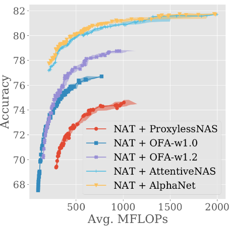
Moreover, there is no supernetwork that covers both very small and very large models.
So the manual choice of a supernetwork restricts what a NAS algorithm can find before the search even starts!
This makes sense, since each supernetwork defines its own search space, with different possible operations, different numbers of layers, and so on.
This also means that subnetworks coming from different supernetworks can be quite diverse. And that’s exactly what we need to create good cascades!
So we can use NAT on each supernetwork separately, and then put all the found models into a single model pool. This way, we can efficiently create many task-specific models that are also diverse because they come from different supernetworks.
How can we search for cascades?
We need several ingredients to define our search procedure.
Solution representation follows the description mentioned above: a cascade of size k can be represented by k models (i.e. the indices of the models in our model pool) and k-1 confidence thresholds (we use indices of discretized values in the [0.0, 1.0] range)
Our multi-objective fitness function estimates the effectivity (e.g. accuracy) and the efficiency (e.g. FLOPs) of a cascade by evaluating it on the validation set.
Any general-purpose multi-objective algorithm can be applied to optimize the fitness function, we use MO-GOMEA, a well-performing EA that requires no hyperparameter tuning (and none was done in our case).
Our algorithm (ENCAS) can be briefly summed up like this:
- (optional) Create diverse models for the specific task by running NAT on many supernetworks.
- Create a combined model pool of all the available models.
- Search for cascades via MO-GOMEA.
ENCAS has several advantages:
- Efficient runtime of 1 GPU-hour thanks to pre-computing the outputs of all the models (which we can do because the models are known in advance).
- Usage of pre-trained weights, which are always important for good performance of neural networks.
- The user only needs to set the maximum cascade size, smaller cascades can still be found. This is achieved by the inclusion of a “no operation” model that does nothing: if a cascade of e.g. size 3 includes this model, it effectively becomes a cascade of size 2.
Experiment setup
We test our approach on CIFAR-10, CIFAR-100, and ImageNet.
Note that for our ImageNet experiments we used additional data for search: we have to do it because search requires data not seen during training, but the pretrained weights that we rely on were trained with all the data. So we use ImageNetV2 for cascade evaluation during the search. Since the size of this additional data is small (it’s just 1.6% of the ImageNet), we hope that the impact of this is negligible.
(also, in our preliminary experiments we tried splitting the ImageNet validation set into two halves - one for the search, and one for reporting the results - and achieved similar results. But since in the literature the results on the whole validation set are usually reported, and we wanted our results to be easy to compare to, we decided to report the results on the whole validation set, and use ImageNetV2 for search).
For all the datasets, the test set was only used to report the results, it was never used to select models, and so some of our trade-off fronts are not monotonous (since the models were selected based on the validation performance, but the test performance is shown).
Each experiment was run 10 times, the median run (by hypervolume) is plotted, and the area between the worst and the best trade-off fronts is shaded.
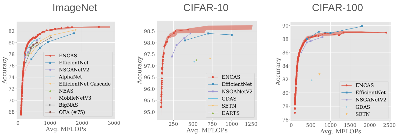
Dominating trade-off front on ImageNet
We ran ENCAS on 518 pre-trained models from timm, which is a brilliant library that includes a wide variety of models that are small (e.g. MobileNetV3@60 MFLOPS), large (e.g. BeiT@362,000 MFLOPS), and everything in between.
ENCAS found a trade-off front of cascades that dominates across the board:
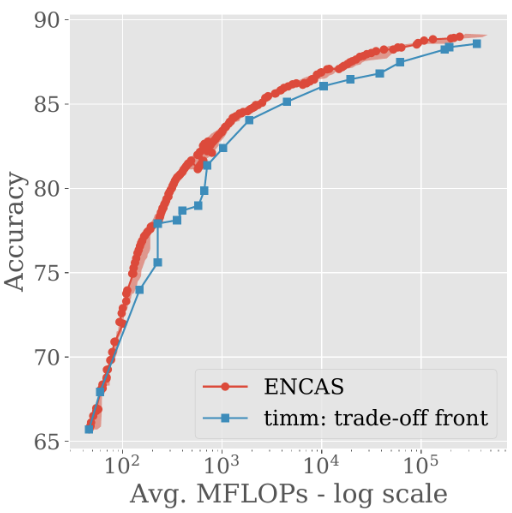
The maximum accuracy was also improved from 88.6% to 89.0%, while the amount of required compute decreased by 18%, from 362 to 296 GFLOPs.
ENCAS finds hundreds of good cascades, which means you can choose one that fits your computational constraints just right.
And all of this was achieved in a single run that took just one GPU-hour! (Well, that’s how long the search itself takes. Prior to it, all the models need to be evaluated, and their outputs stored, which takes some hours, but only needs to be done once)
The ability to work in a search space of hundreds of models is important for great results. In the previous work that strongly inspired us, cascades of EfficientNet models were found via grid search.
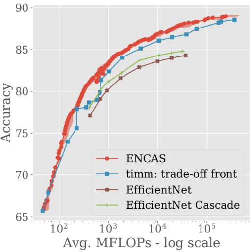
The resulting cascades improve the trade-off front, but it’s hard to go beyond the models available in the pool (which motivates making the pool as large as possible, which in turn prohibits the usage of inefficient approaches like grid search (to be clear, the authors of the work point it out themselves; the search algorithm was not the key part of that work)).
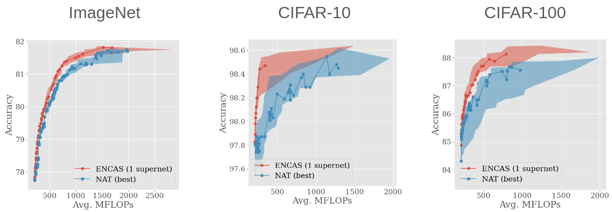
NAS-discovered networks are improved by cascading
We applied our implementation of NAT to 5 supernetworks, and chose the one that produced the best trade-off front. Then we ran ENCAS on the models from this front, and achieved better trade-off fronts for all the datasets!
Five supernetworks are better than one
We then applied ENCAS to the trade-off fronts of all five supernetworks instead of just the best one, and the results improved even more:
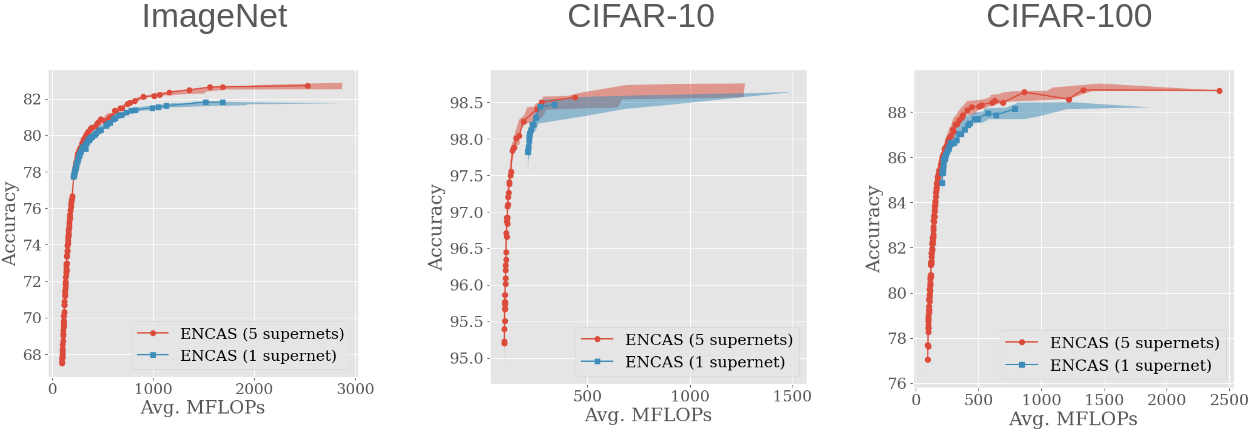
This means that increasing the size & diversity of the model pool improves the results. Our method is able to work with models from arbitrary supernetworks, and thus make use of diverse & incompatible search spaces.
(But I should mention that currently available supernetworks are not very diverse, and so the impact is not as big as it could be - see the paper for further discussion of this and other limitations)
Still, the current good results mean that…
ENCAS outperforms efficient NAS approaches
(in most cases)
This is achieved in large part thanks to cascades and to the availability of ImageNet-pretrained supernetworks that NAT can effectively adapt to the task at hand, thus creating a good model pool for ENCAS.
Conclusion
The main strength of ENCAS is its generality: any trade-off front of models can be improved by cascading - it doesn’t matter where the models came from. For example, it would be possible to outperform EfficientNet-s on CIFAR-100 by simply adding these models to the model pool of the NAT-derived models.
This means that you need to simply get many models in any way you want, and then just let the search find good cascades for you, making the model on your trade-off front more effective and efficient.
Our code is publicly available, so I invite you to try it out for yourself.
The paper contains more cool experiments (e.g. joint supernetwork weight adaptation and cascade architecture search) - check it out if you’re interested!
To cite:
@inproceedings{10.1145/3512290.3528749,
	author = {Chebykin, Alexander and Alderliesten, Tanja and Bosman, Peter A. N.},
	title = {Evolutionary Neural Cascade Search across Supernetworks},
	year = {2022},
	isbn = {9781450392372},
	publisher = {Association for Computing Machinery},
	address = {New York, NY, USA},
	url = {https://doi.org/10.1145/3512290.3528749},
	doi = {10.1145/3512290.3528749},
	booktitle = {Proceedings of the Genetic and Evolutionary Computation Conference},
	pages = {1038–1047},
	numpages = {10},
	series = {GECCO '22}
}